In this week’s blog post I will explore how demographics provide insight into the electorate and election outcomes.
## Confusion Matrix and Statistics
##
##             Reference
## Prediction   Democrat Republican
##   Democrat        746        336
##   Republican      346        660
##
##                Accuracy : 0.6734
##                  95% CI : (0.6528, 0.6935)
##     No Information Rate : 0.523
##     P-Value [Acc > NIR] : <2e-16
##
##                   Kappa : 0.3456
##
##  Mcnemar's Test P-Value : 0.7304
##
##             Sensitivity : 0.6832
##             Specificity : 0.6627
##          Pos Pred Value : 0.6895
##          Neg Pred Value : 0.6561
##              Prevalence : 0.5230
##          Detection Rate : 0.3573
##    Detection Prevalence : 0.5182
##       Balanced Accuracy : 0.6729
##
##        'Positive' Class : Democrat
##
##Replicating Kim & Zilinsky (2023)
Kim & Zilinsky (2023) co-authored a paper where they concluded that demographic information (five key attributes) about a voter can accurately predict a voter’s choice with an accuracy of 63.9%.
The replication above corroborates Kim & Zilinsky’s findings. The 95% confidence interval ranges from 65.28% to 69.35%. I personally found this interesting because campaigns reach out to likely voters based on demographic information. It makes sense for a campaign with limited resources to make an educated guess on who to target based on a voter’s demographics. Not only that, but when election predictions are being made, the demographics of the electorate are frequently cited.
Demographic attributes like race are constantly in the headlines. In one CBS article, the headline reads “Kamala Harris turns to her faith in outreach to Black voters” One quote from the article highlights the importance of reaching out to Black voters, “Her focus underscores the importance for her in activating and persuading Black voters, the core of her party’s electorate, by going to a stronghold within the community.”
In a country where race impacts the quality of life and experience of the voter, it makes sense for race to indicate a partisan preference. Especially when we consider political polarization in a two-party system.
Call: glm(formula = voted_2020 ~ sii_age_range + sii_gender + sii_race + sii_education_level, family = binomial, data = tx_fl)
| Log odds | Probabilities | |
|---|---|---|
| Intercept | -1.2141138 | 0.2289740 |
| Age Range 30-39 | 0.7860256 | 0.6869773 |
| Age Range 40-49 | 1.0305721 | 0.7370268 |
| Age Range 50-64 | 1.2070943 | 0.7697844 |
| Age Range 65-74 | 1.4014692 | 0.8024169 |
| Age Range 75+ | 1.0439784 | 0.7396169 |
| Male | -0.2827494 | 0.4297799 |
| Expansive | -0.3438069 | 0.4148850 |
| Unknown1 | 1.5734212 | 0.8282708 |
| African-American | 0.1872100 | 0.5466663 |
| Hispanic | -0.1463079 | 0.4634881 |
| Native American | 0.2790825 | 0.5693213 |
| Other | 0.7097148 | 0.6703381 |
| Unknown2 | -0.6246810 | 0.3487176 |
| Caucasian | 0.5452111 | 0.6330238 |
| Some College or Higher | 0.7302751 | 0.6748656 |
| Completed College | 1.0250856 | 0.7359620 |
| Completed Graduate School | 0.6770579 | 0.6630817 |
| Attended Vocational/Technical | 0.4725291 | 0.6159822 |


| sii_gender | count | percentage |
|---|---|---|
| Expansive | 5 | 0.0021983 |
| Female | 113230 | 49.7832453 |
| Male | 107620 | 47.3167257 |
| Unknown | 6591 | 2.8978307 |
| sii_age_range | count | percentage |
|---|---|---|
| 18-29 | 41925 | 18.43295 |
| 30-39 | 39333 | 17.29334 |
| 40-49 | 37634 | 16.54635 |
| 50-64 | 53892 | 23.69442 |
| 65-74 | 29703 | 13.05936 |
| 75+ | 24959 | 10.97359 |
##Analyzing the Texas Voter File
To explore what insights we can obtain from voter demographics, I will analyze the Texas voter file.
I ran a binomial logistic regression to estimate the relationship between whether a voter voted in 2020 and age range, race, gender, and education level. These are four out of the five attributes Kim and Zilinsky used for their random forest model. I don’t have information about each voter’s income in the file.
The binomial logistic regression models how the probability of success varies with the independent variables and helps determines whether the changes are statistically significant. In this case, success is defined as the person voting. The binomial logistic regression produces the logarithm of the odds as shown in the table. It’s not simple to interpret and visualize the logarithm of the odds so I converted into probabilities.
Essentially what I can takeaway from this regression is that the intercept is the baseline log-odds of voting for the reference group. In this case it is the age range 18-29, females, Asian voters, and the completed high school categories. The Unknowns in the table represent when the voter file had marked unknown race and gender for the voter. Since the unknowns do not represent a specific demographic I will ignore their associated values in my analysis.
The intercept of -1.21 is the log odds of voting for the reference groups, which are age group 18-29, female gender, Asian, and completed high school. The log-odds can be converted to probabilities by raising e to the log-odds and and dividing it by 1 + e raised to the value of the log-odds.
The age range odds and probabilities demonstrate that older citizens tend to vote in higher rates. In this sample of Texas voters, the age range with the highest turnout is 65 to 74. This is consistent with the available literature on age and voter turnout.
Males and the other genders in this Texas voter file have negative log-odds which means that every other category in this sample have lower odds of voting compared to female voters. This too is also consistent with the available data on voter turnout (Gender differences in voter turnout)
All races except Hispanic have a positive coefficient, indicating that Hispanics have lower odds and probabilities of voting than the baseline group (Asians). It is unclear what demographics are represented under the Other category but the next group with highest odds are Caucasian.
When looking at education, it is consistent with available data and literature that those who have completed college and graduate school are the groups of registered voters with the highest odds of voting.
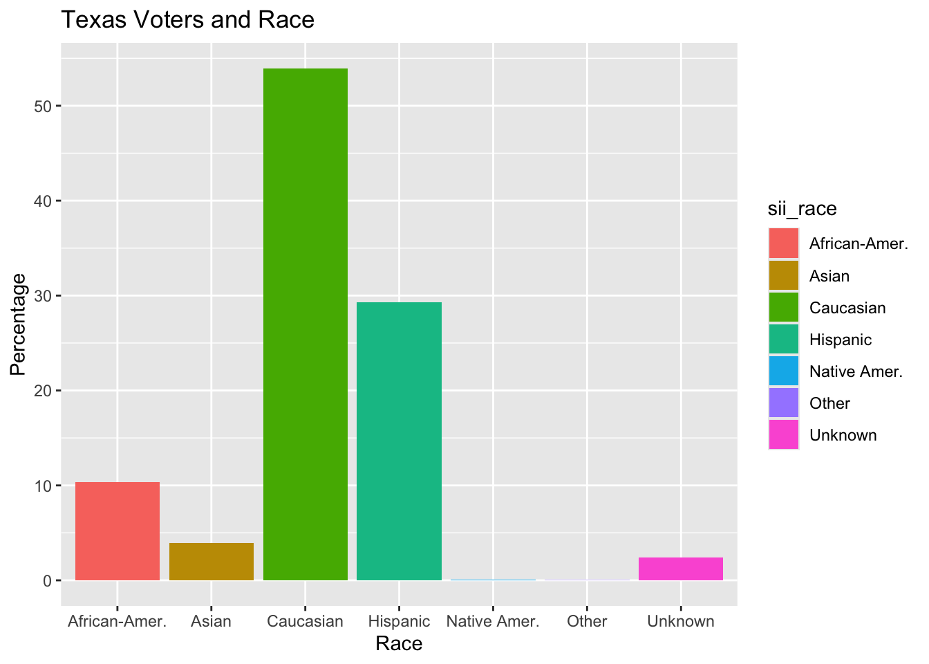
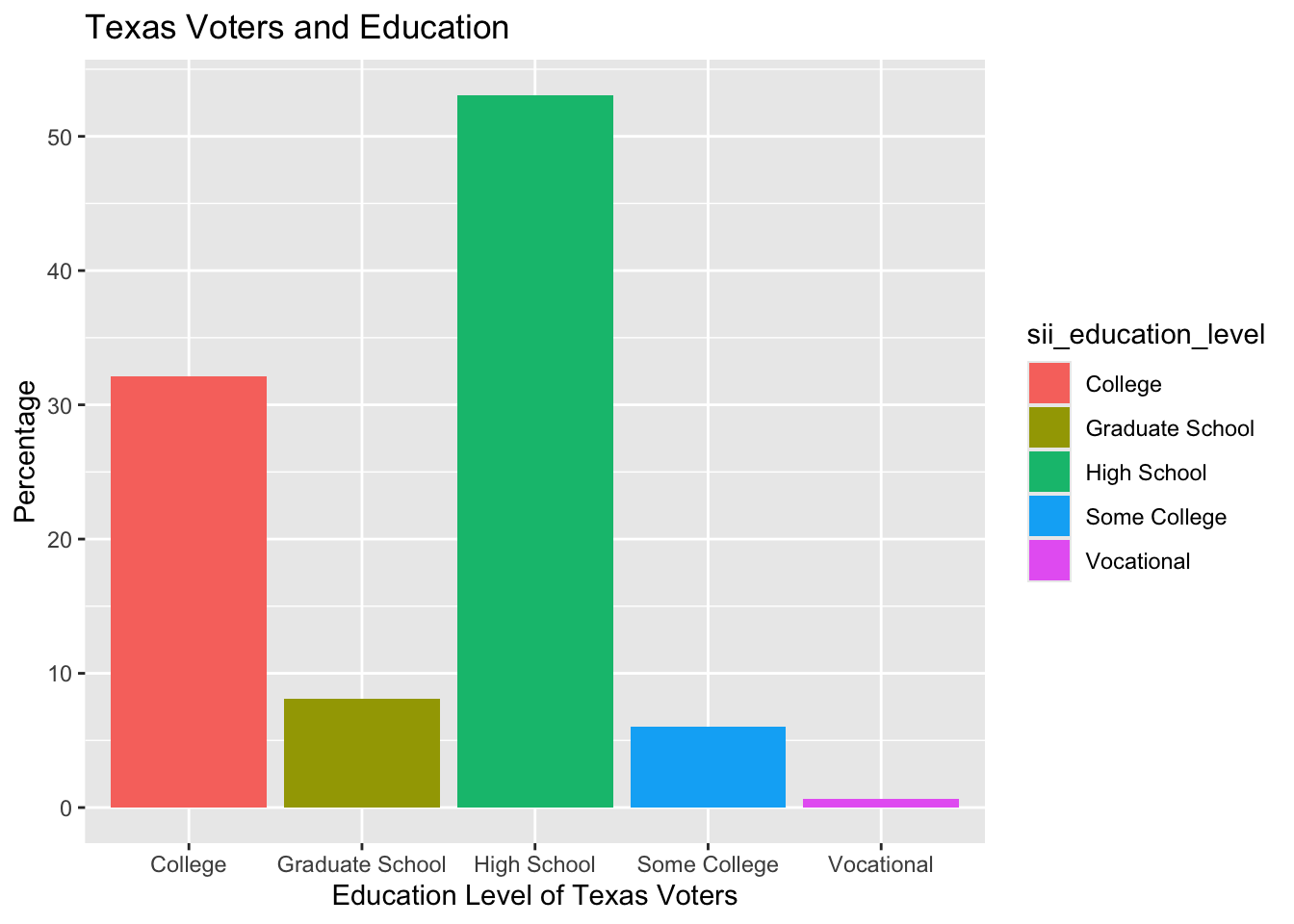
I have also included some graphs that provide descriptive statistics about the Texas electorate. The majority of registered voters in Texas is Caucasian, making up about 53% of registered voters. The next largest group is Hispanic voters, making up just under 30% of registered voters.
Most of the Texas electorate completed high school and college. In regard to gender, there is an almost 50-50 split between female and male registered voters. The age range group leading in registered voters is 50-64, followed by 18-29. Although the 18-29 age range is known for being the age range with the lowest voter turnout.
##Simulation and Prediction for this Week
| party | total_electors |
|---|---|
| Democrat | 319 |
| Republican | 219 |

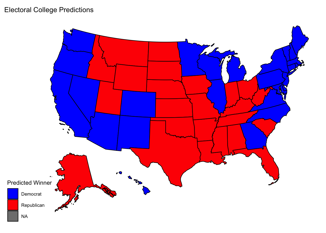
My prediction for this week is based on a simple linear model that uses polling data, two-party lagged vote shares, and turnout data. 10,000 simulations are then run to account for variability in turnout. One of the benefits of simulating with turnout variability is that it provides a range of plausible turnout percentages which captures how changes in voter turnout across states can influence the election outcome. The final prediction is that Kamala Harris wins 319 electors and Trump wins 219. This model predicts that Harris will win in all the swing states which is an interesting result that I am hesitant about accepting but provokes thoughts about how to refine this model for future iterations.
##References
“Gender Differences in Voter Turnout.” Center for American Women and Politics, cawp.rutgers.edu/facts/voters/gender-differences-voter-turnout. Accessed 28 Oct. 2024.
Kim, Seo-young Silvia, and Jan Zilinsky. “Division Does Not Imply Predictability: Demographics Continue to Reveal Little about Voting and Partisanship.” Political Behavior, vol. 46, no. 1, 20 Aug. 2022, pp. 67–87, doi:10.1007/s11109-022-09816-z.
Navarro, Aaron. “Kamala Harris Turns to Her Faith in Outreach to Black Voters.” CBS News, CBS Interactive, www.cbsnews.com/news/kamala-harris-faith-black-voter-outreach/. Accessed 27 Oct. 2024.