@title GOV 1347: Week 2 (Economics) Laboratory Session @author Matthew E. Dardet @date September 10, 2024
Date: September, 16, 2024
This Week’s Question: Can we predict election outcomes using only the state of the economy? If so, how well?
## Loading required package: carData
## ── Attaching core tidyverse packages ──────────────────────── tidyverse 2.0.0 ──
## ✔ dplyr     1.1.4     ✔ readr     2.1.5
## ✔ forcats   1.0.0     ✔ stringr   1.5.1
## ✔ ggplot2   3.5.1     ✔ tibble    3.2.1
## ✔ lubridate 1.9.3     ✔ tidyr     1.3.1
## ✔ purrr     1.0.2
## ── Conflicts ────────────────────────────────────────── tidyverse_conflicts() ──
## ✖ dplyr::filter() masks stats::filter()
## ✖ dplyr::lag()    masks stats::lag()
## ✖ dplyr::recode() masks car::recode()
## ✖ purrr::some()   masks car::some()
## ℹ Use the conflicted package (<http://conflicted.r-lib.org/>) to force all conflicts to become errors
####———————————————————-#
Read, merge, and process data.
####———————————————————-#
## Rows: 38 Columns: 9
## ── Column specification ────────────────────────────────────────────────────────
## Delimiter: ","
## chr (2): party, candidate
## dbl (3): year, pv, pv2p
## lgl (4): winner, incumbent, incumbent_party, prev_admin
##
## ℹ Use `spec()` to retrieve the full column specification for this data.
## ℹ Specify the column types or set `show_col_types = FALSE` to quiet this message.
## Rows: 387 Columns: 14
## ── Column specification ────────────────────────────────────────────────────────
## Delimiter: ","
## dbl (14): year, quarter, GDP, GDP_growth_quarterly, RDPI, RDPI_growth_quarte...
##
## ℹ Use `spec()` to retrieve the full column specification for this data.
## ℹ Specify the column types or set `show_col_types = FALSE` to quiet this message.
## Rows: 310 Columns: 11
## ── Column specification ────────────────────────────────────────────────────────
## Delimiter: ","
## chr  (1): Quarter
## dbl (10): Year, Gross domestic product, Gross national product, Disposable p...
##
## ℹ Use `spec()` to retrieve the full column specification for this data.
## ℹ Specify the column types or set `show_col_types = FALSE` to quiet this message.
## Joining with `by = join_by(year)`
## Joining with `by = join_by(year)`
####———————————————————-#
Understanding the relationship between economy and vote share.
####———————————————————-#
## [1] 0.4336956
##
## Call:
## lm(formula = pv2p ~ GDP_growth_quarterly, data = d_inc_econ)
##
## Residuals:
##     Min      1Q  Median      3Q     Max
## -6.7666 -3.3847 -0.7697  2.9121  8.8809
##
## Coefficients:
##                      Estimate Std. Error t value Pr(>|t|)
## (Intercept)           51.2580     1.1399  44.968   <2e-16 ***
## GDP_growth_quarterly   0.2739     0.1380   1.985   0.0636 .
## ---
## Signif. codes:  0 '***' 0.001 '**' 0.01 '*' 0.05 '.' 0.1 ' ' 1
##
## Residual standard error: 4.834 on 17 degrees of freedom
## Multiple R-squared:  0.1881,	Adjusted R-squared:  0.1403
## F-statistic: 3.938 on 1 and 17 DF,  p-value: 0.06358
##
## Call:
## lm(formula = pv2p ~ GDP_growth_quarterly, data = d_inc_econ_2)
##
## Residuals:
##    Min     1Q Median     3Q    Max
## -6.237 -4.160  0.450  1.904  8.728
##
## Coefficients:
##                      Estimate Std. Error t value Pr(>|t|)
## (Intercept)           49.3751     1.4163  34.862   <2e-16 ***
## GDP_growth_quarterly   0.7366     0.2655   2.774   0.0135 *
## ---
## Signif. codes:  0 '***' 0.001 '**' 0.01 '*' 0.05 '.' 0.1 ' ' 1
##
## Residual standard error: 4.463 on 16 degrees of freedom
## Multiple R-squared:  0.3248,	Adjusted R-squared:  0.2826
## F-statistic: 7.697 on 1 and 16 DF,  p-value: 0.01354
## Warning: The following aesthetics were dropped during statistical transformation: label.
## ℹ This can happen when ggplot fails to infer the correct grouping structure in
##   the data.
## ℹ Did you forget to specify a `group` aesthetic or to convert a numerical
##   variable into a factor?
## Warning: The following aesthetics were dropped during statistical transformation: label.
## ℹ This can happen when ggplot fails to infer the correct grouping structure in
##   the data.
## ℹ Did you forget to specify a `group` aesthetic or to convert a numerical
##   variable into a factor?
## [1] 0.3248066
## [1] 0.282607
##        1
## 28.75101
## # A tibble: 1 × 1
##    pv2p
##   <dbl>
## 1  47.7
##        pv2p
## 1 -18.97913
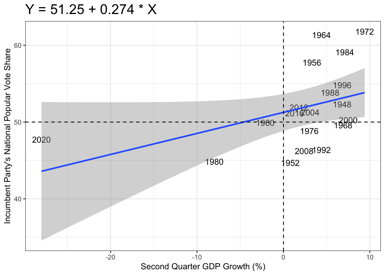
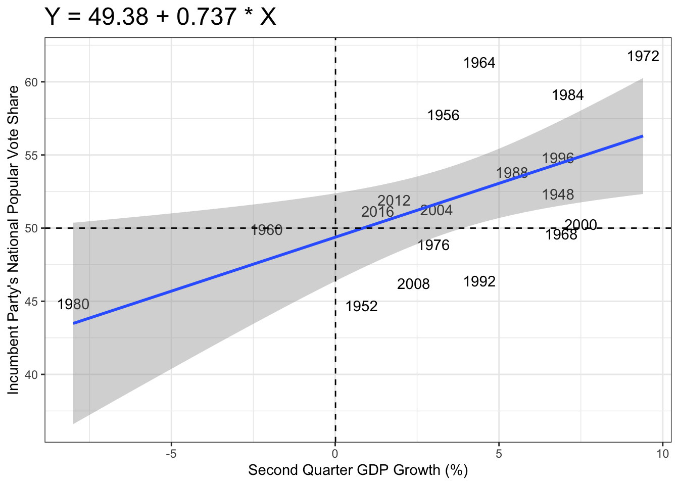
The graphs demonstrate the correlations between Q2 GDP growth and incumbent vote 2-party vote share. One with 2020 as a data point and one without 2020 as a data point. Regardless, both graphs demonstrate the same trend, an increase in GDP in Q2 does correlate positively with an increase in the total vote share for the incumbent. What is interesting to point out is that when 2020 is removed as a data point the “slope” for GDP growth quarterly increases. It’s coefficient is 0.7366 compared to 0.274 before removing 2020 as a data point which indicates to me that the GDP growth quarterly might be an outlier. A survey conducted by the Pew Research Center in 2020 shows that the top issue for voters in 2020 was the economy, which makes sense because 2020 was peak pandemic time and many had lost their job or had reduced hours. Additionally many Americans stayed home to mitigate the spread of COVID-19 but despite the importance of the economy, the incumbent overperformed despite the lowest GDP growth for Q2 in the past 80 years (https://www.pewresearch.org/politics/2020/08/13/important-issues-in-the-2020-election/). When looking at the graph above, the the incumbent received more of the total vote share than predicted. Generally though the trend exists but is not very strong because the adjusted R-squared value is 0.2826 whereas a 0.50 to 0.99 indicates greater fit.
##
## Call:
## lm(formula = pv2p ~ unemployment, data = d_inc_econ_unemployment)
##
## Residuals:
##     Min      1Q  Median      3Q     Max
## -7.9906 -2.6616 -0.9256  2.4016  9.9399
##
## Coefficients:
##              Estimate Std. Error t value Pr(>|t|)
## (Intercept)   53.6260     3.4614  15.493 1.85e-11 ***
## unemployment  -0.3117     0.5475  -0.569    0.577
## ---
## Signif. codes:  0 '***' 0.001 '**' 0.01 '*' 0.05 '.' 0.1 ' ' 1
##
## Residual standard error: 5.314 on 17 degrees of freedom
## Multiple R-squared:  0.01872,	Adjusted R-squared:  -0.03901
## F-statistic: 0.3243 on 1 and 17 DF,  p-value: 0.5765
## Warning: The following aesthetics were dropped during statistical transformation: label.
## ℹ This can happen when ggplot fails to infer the correct grouping structure in
##   the data.
## ℹ Did you forget to specify a `group` aesthetic or to convert a numerical
##   variable into a factor?
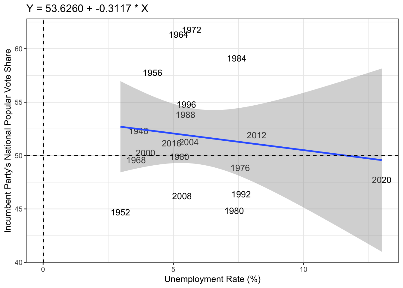
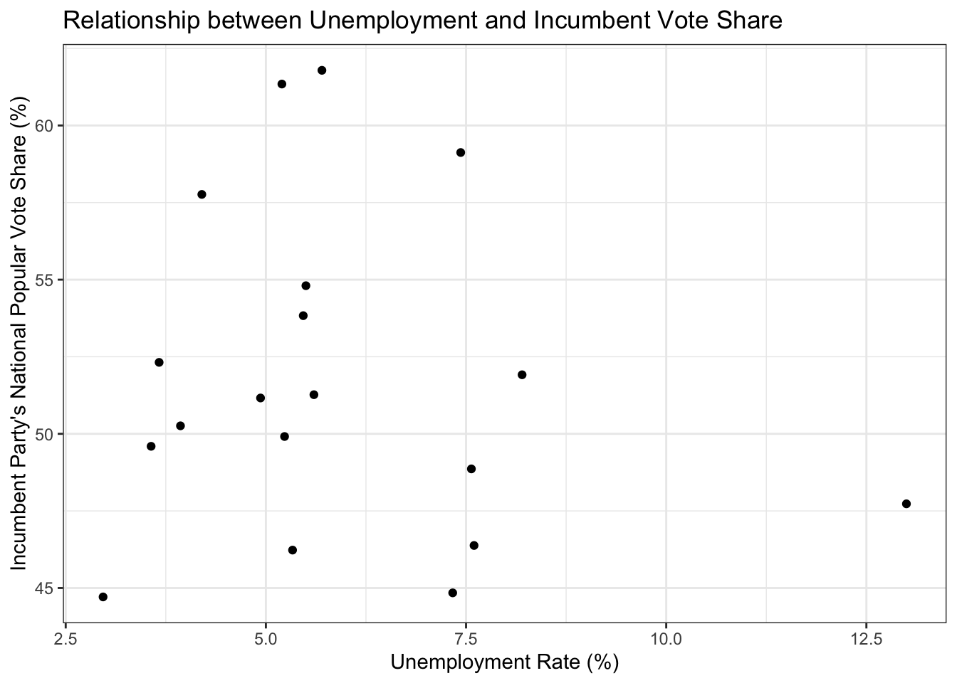
In the graph above, I performed an analysis on the correlation between the unemployment rate and the incumbent party’s national popular vote share (%). What I found was a model that indicates that for every increase in 1% of unemployment, the incumbent party loses -0.3117 of a point in total vote share. The 2020 data point again seems to be an outlier and drags the trend down but without this data point there would be less correlation. The adjusted r-square value is -0.03901 which indicates that the unemployment rate does not explain much of the variation and thus this variable has a weak influence on the total vote share. However, I did find this journal article that argues that employment security is a powerful indicator of economic performance and thus the increase in unemployment should result in decrease of support for the incumbent. “Employment Insecurity, Incumbent Partisanship, and Voting Behavior in Comparative Perspective” (https://journals.sagepub.com/doi/10.1177/0010414016679176) I was surprised to see that there was not a stronger association because candidates and elected officials often tout the creation of new jobs.
##
## Call:
## lm(formula = pv2p ~ RDPI_growth_quarterly, data = d_inc_econ)
##
## Residuals:
##     Min      1Q  Median      3Q     Max
## -7.2308 -2.9971 -0.8344  2.4629  9.9337
##
## Coefficients:
##                       Estimate Std. Error t value Pr(>|t|)
## (Intercept)           51.97420    1.49322  34.807   <2e-16 ***
## RDPI_growth_quarterly -0.02831    0.12446  -0.227    0.823
## ---
## Signif. codes:  0 '***' 0.001 '**' 0.01 '*' 0.05 '.' 0.1 ' ' 1
##
## Residual standard error: 5.357 on 17 degrees of freedom
## Multiple R-squared:  0.003033,	Adjusted R-squared:  -0.05561
## F-statistic: 0.05172 on 1 and 17 DF,  p-value: 0.8228
## Warning: The following aesthetics were dropped during statistical transformation: label.
## ℹ This can happen when ggplot fails to infer the correct grouping structure in
##   the data.
## ℹ Did you forget to specify a `group` aesthetic or to convert a numerical
##   variable into a factor?
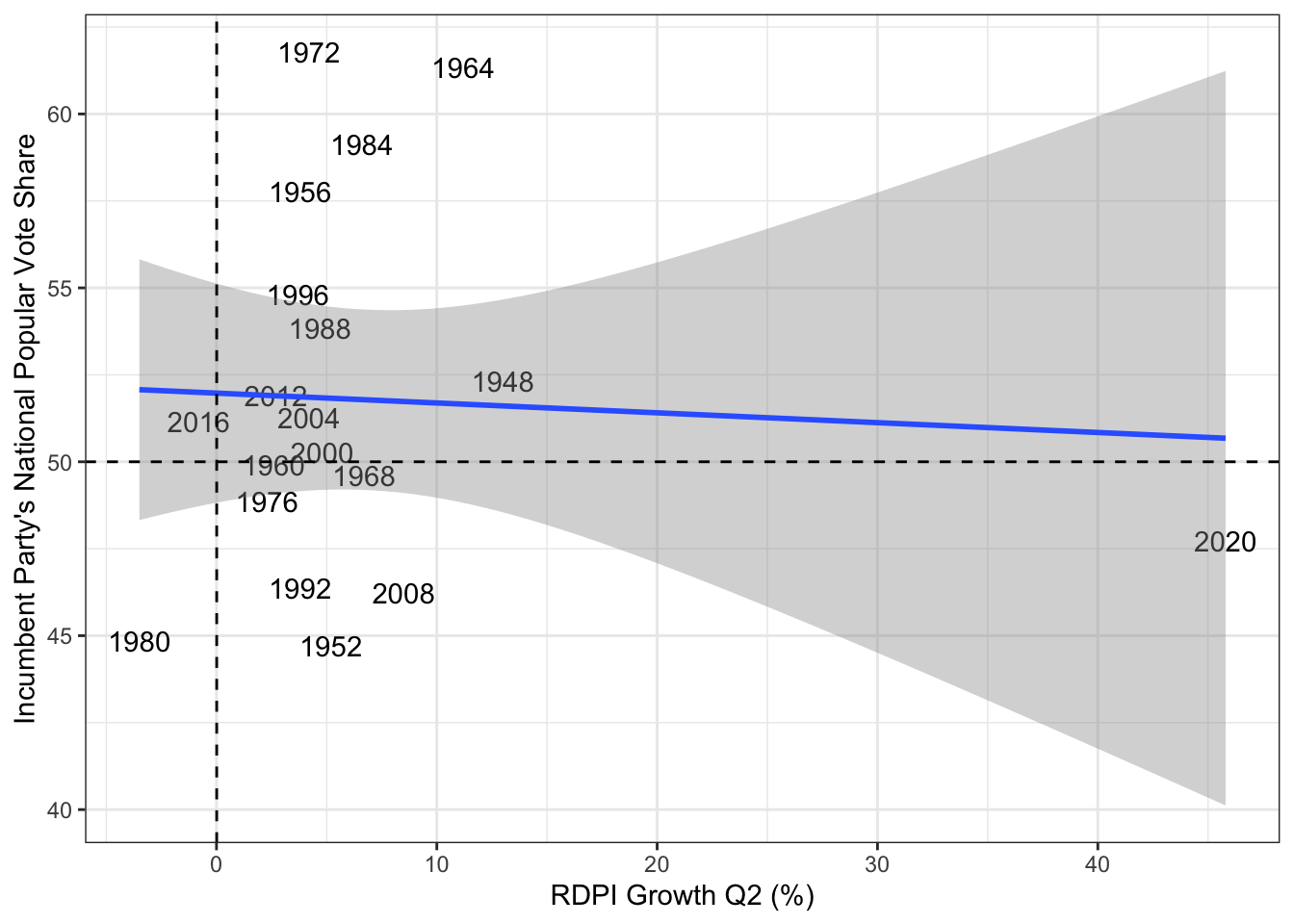
The graph above demonstrates the real disposable personal income (RDPI) growth in Q2 and its correlation with the incumbent party’s national popular vote share. Visually it appears that there is not a strong correlation because it looks like a lot of the dates are stacked in the graph which means that even when RDPI is similar the vote share can vary quite a bit from 45 to almost 60 percent of the vote share if you look at year 1952 and 1984. This is supported by the weak association that the linear regression model provided. The adjusted r-squared value is -0.05561 which is relatively low. Again, the 2020 data point seems to be an outlier. I wonder if the reason why real disposable income may not have a strong effect on the incumbent party’s vote share has to do with the fact that people can still purchase items they can’t afford by placing it on credit cards and therefore they don’t necessarily feel as though their disposable income is severely affected. The federal bank reserve of New York reports that household debt is up to $17.80 trillion in second quarter (https://www.newyorkfed.org/microeconomics/hhdc).
####———————————————————-#
Predicting 2024 results using simple economy model.
####———————————————————-#
##        1
## 51.58486
##        1
## 52.37907
##       1
## 51.9459
##        fit      lwr     upr
## 1 51.58486 41.85982 61.3099
##        fit      lwr      upr
## 1 52.37907 40.66441 64.09372
##       fit      lwr      upr
## 1 51.9459 40.25082 63.64097
Above are the predicted values and intervals for the incumbent party’s vote share with the unemployment rate from and RDPI Q2 growth from 2024 respectively.
To answer this week’s question, about how well we can predict election outcomes using only the state of the economy I can say that RDPI from Q2 and the unemployment rate are not enough to predict the election well enough because there was not a strong association between those variables and the incumbent party’s vote share as shown visually by the graphs and r-squared values. Additionally, the national popular vote share is not indicative of the election winner because that is determined by the electoral college although usually the winner tends to win the popular vote. Where I would go from here is looking at other economy indicators and perhaps even go state by state to see who wins in that state and then use information that to calculate the electoral college count.