Welcome to my election blog! Every week I will be updating my election model and providing analysis to forecast the outcome of the 2024 presidential election as part of an assignment for GOV 1347.
The following template is created by Matthew Dardet. In the following weeks I will be building off this election model from our lab section.
This week I aim to answer the following questions:
- How competitive are presidential elections in the United States?
- Which states vote blue/red and how consistently?
## ── Attaching core tidyverse packages ──────────────────────── tidyverse 2.0.0 ──
## ✔ dplyr     1.1.4     ✔ readr     2.1.5
## ✔ forcats   1.0.0     ✔ stringr   1.5.1
## ✔ lubridate 1.9.3     ✔ tibble    3.2.1
## ✔ purrr     1.0.2     ✔ tidyr     1.3.1
## ── Conflicts ────────────────────────────────────────── tidyverse_conflicts() ──
## ✖ dplyr::filter() masks stats::filter()
## ✖ dplyr::lag()    masks stats::lag()
## ✖ purrr::map()    masks maps::map()
## ℹ Use the conflicted package (<http://conflicted.r-lib.org/>) to force all conflicts to become errors
## Rows: 38 Columns: 9
## ── Column specification ────────────────────────────────────────────────────────
## Delimiter: ","
## chr (2): party, candidate
## dbl (3): year, pv, pv2p
## lgl (4): winner, incumbent, incumbent_party, prev_admin
##
## ℹ Use `spec()` to retrieve the full column specification for this data.
## ℹ Specify the column types or set `show_col_types = FALSE` to quiet this message.
## [1] "year"            "party"           "winner"          "candidate"
## [5] "pv"              "pv2p"            "incumbent"       "incumbent_party"
## [9] "prev_admin"
## # A tibble: 2 × 3
##   party      candidate         pv2p
##   <chr>      <chr>            <dbl>
## 1 democrat   Biden, Joseph R.  52.3
## 2 republican Trump, Donald J.  47.7
## # A tibble: 19 × 3
##     year democrat republican
##    <dbl>    <dbl>      <dbl>
##  1  1948     52.3       47.7
##  2  1952     44.7       55.3
##  3  1956     42.2       57.8
##  4  1960     50.1       49.9
##  5  1964     61.3       38.7
##  6  1968     49.6       50.4
##  7  1972     38.2       61.8
##  8  1976     51.1       48.9
##  9  1980     44.8       55.2
## 10  1984     40.9       59.1
## 11  1988     46.2       53.8
## 12  1992     53.6       46.4
## 13  1996     54.8       45.2
## 14  2000     50.3       49.7
## 15  2004     48.7       51.3
## 16  2008     53.8       46.2
## 17  2012     51.9       48.1
## 18  2016     51.2       48.8
## 19  2020     52.3       47.7
## # A tibble: 19 × 4
##     year democrat republican winner
##    <dbl>    <dbl>      <dbl> <chr>
##  1  1948     52.3       47.7 D
##  2  1952     44.7       55.3 R
##  3  1956     42.2       57.8 R
##  4  1960     50.1       49.9 D
##  5  1964     61.3       38.7 D
##  6  1968     49.6       50.4 R
##  7  1972     38.2       61.8 R
##  8  1976     51.1       48.9 D
##  9  1980     44.8       55.2 R
## 10  1984     40.9       59.1 R
## 11  1988     46.2       53.8 R
## 12  1992     53.6       46.4 D
## 13  1996     54.8       45.2 D
## 14  2000     50.3       49.7 D
## 15  2004     48.7       51.3 R
## 16  2008     53.8       46.2 D
## 17  2012     51.9       48.1 D
## 18  2016     51.2       48.8 D
## 19  2020     52.3       47.7 D
## # A tibble: 2 × 2
##   winner races
##   <chr>  <int>
## 1 D         11
## 2 R          8
####----------------------------------------------------------#
#### Visualize trends in national presidential popular vote.
####----------------------------------------------------------#

# Visualize the two-party presidential popular over time.

d_popvote |>
  ggplot(aes(x = year, y = pv2p, color = party)) +
  geom_line() +
  scale_color_manual(values = c("dodgerblue4", "firebrick1")) +
  labs(title = "two-party presidential popular over time",
        x = "year",
        y = "2p vote prop.") +
  theme_bw()
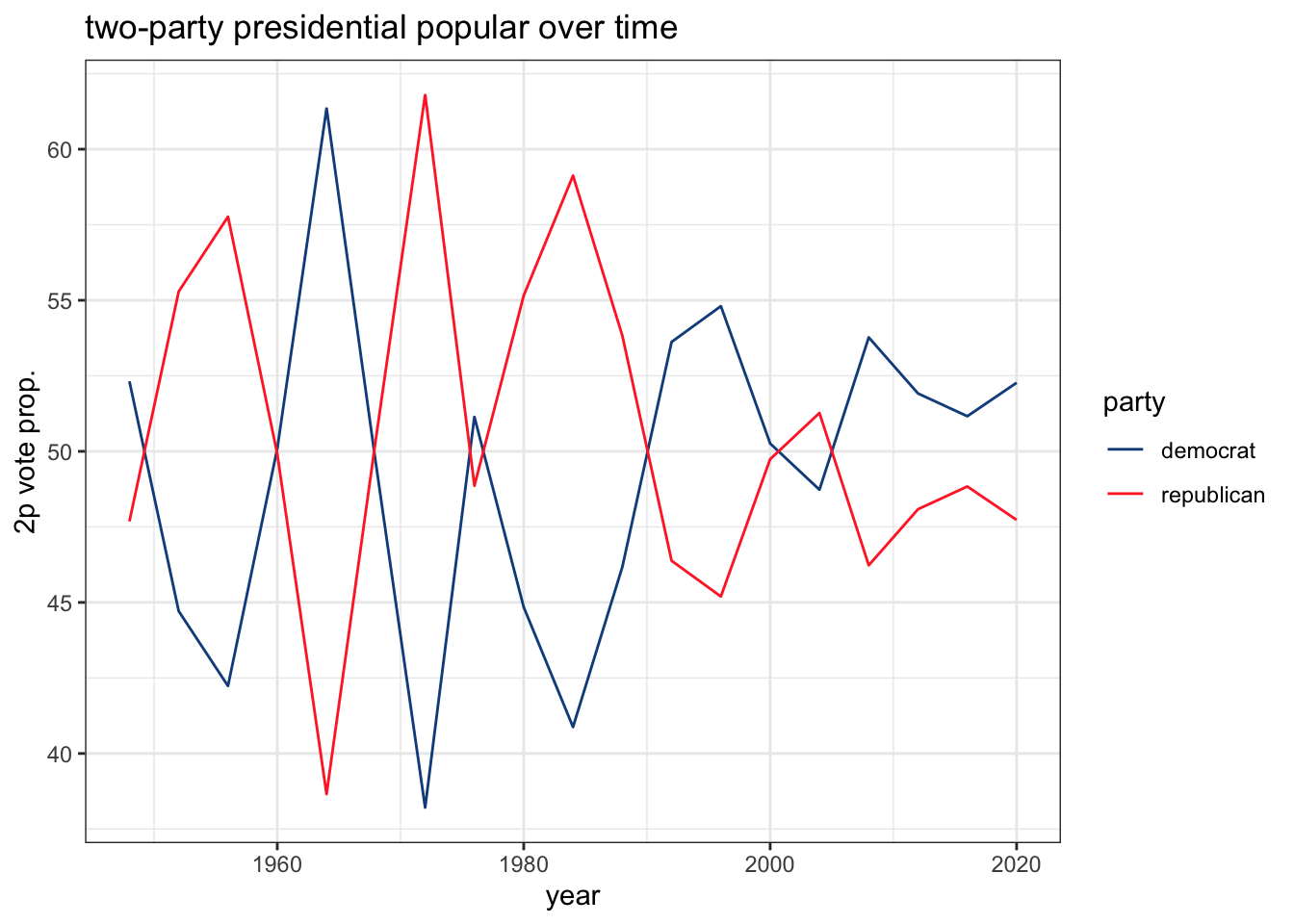
This graph can help us understand how competitive U.S. presidential elections are because it demonstrates the proportion of popular vote Democrats and Republican presidential candidates have obtained. It is important to note that elections are not won by popular vote but it is not unreasonable to presume that the elected presidents do not tend to win the popular vote. A document posted by the Alabama Secretary of State (https://www.sos.alabama.gov/sites/default/files/election-data/Electoral%20College%20FAQ.pdf) notes that only four times throughout American history has a president won the election without the popular vote. The 2016 presidential election is one of those outliers as displayed by the graph. Hilary Clinton obtained won the popular vote and lost the electoral college thus costing her the presidency.
Additionally, it is worth mentioning that this data displays the two party popular vote share which excludes third party candidates that have made it onto the ballot. American presidential elections are competitive if the candidate is on the Democratic or Republican presidential ticket, leaving small opportunity for other party candidates.
A visual analysis of the graph above shows that over time American voters have let both parties have presidential power and the fact that it does swing and change over years highlights competitiveness. In fact it appears that elections are getting more competitive. Between 1950 and 1990 the difference between the proportion of the popular vote is wider than than it has been in the past 30 years. The difference is getting smaller which indicates that elections are becoming more competitive because both parties are getting closer in popular vote proportions.
## Rows: 959 Columns: 14
## ── Column specification ────────────────────────────────────────────────────────
## Delimiter: ","
## chr  (1): state
## dbl (13): year, D_pv, R_pv, D_pv2p, R_pv2p, D_pv_lag1, R_pv_lag1, D_pv2p_lag...
##
## ℹ Use `spec()` to retrieve the full column specification for this data.
## ℹ Specify the column types or set `show_col_types = FALSE` to quiet this message.
## Warning in left_join(filter(d_pvstate_wide, year >= 1980), states_map, by = "region"): Detected an unexpected many-to-many relationship between `x` and `y`.
## ℹ Row 1 of `x` matches multiple rows in `y`.
## ℹ Row 1 of `y` matches multiple rows in `x`.
## ℹ If a many-to-many relationship is expected, set `relationship =
##   "many-to-many"` to silence this warning.
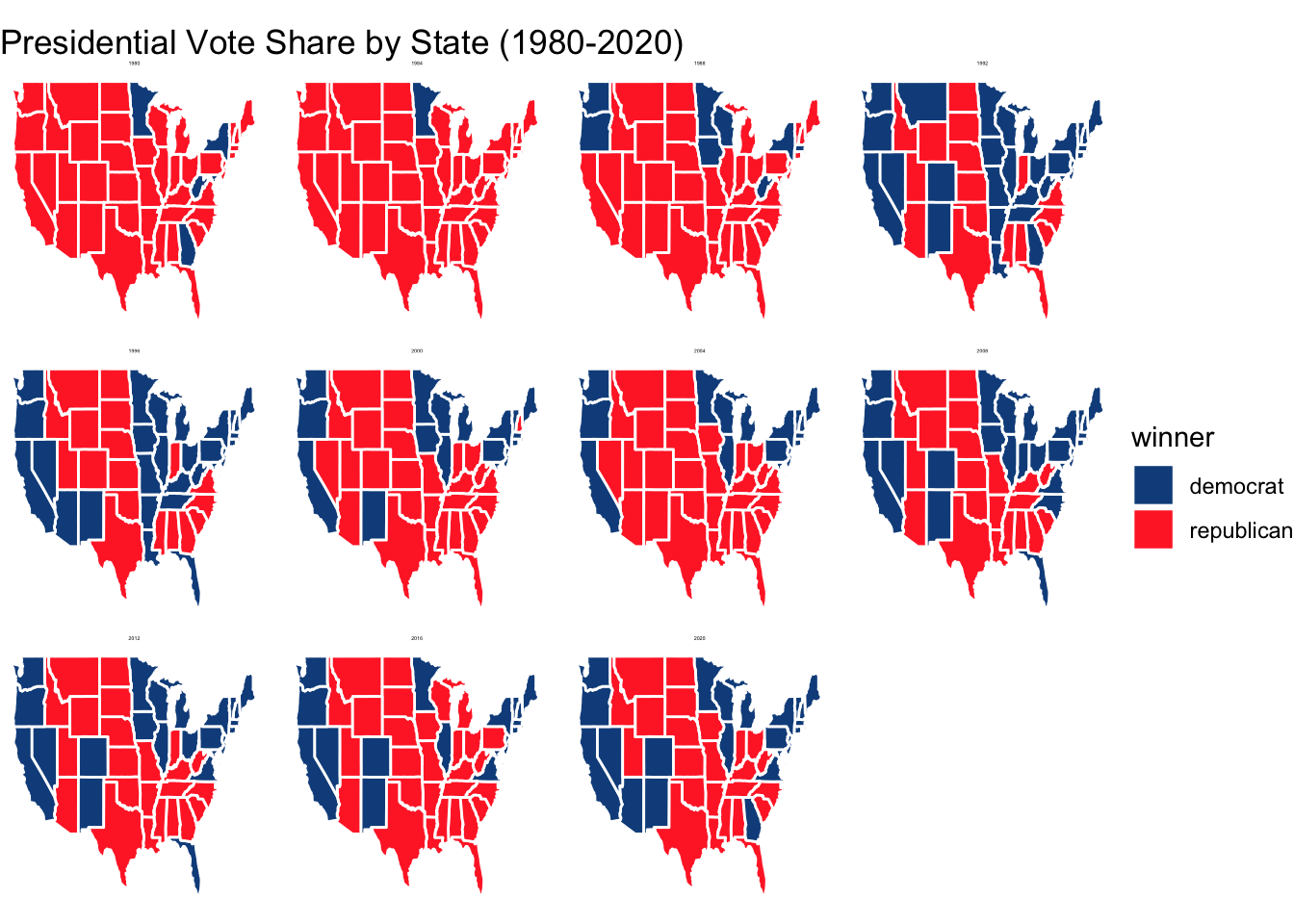
This grid map of which party candidate won each state between 1980 and 2020 further supports the idea that elections have become more competitive. In 1980 and 1984, the maps are mostly red, indicating that one candidate won by a large margin of electoral college votes. After the 1988 election, the Democratic candidate starts winning states. Beyond the 1992 election, the Democratic candidate picks up states that are considered strongholds for them such as California, New York, Illinois, and a batch of northeast states. Minnesota, Washington and Oregon also prove to be consistently voting for the Democratic candidate. This grid map also shows that southern U.S. and west (excluding coastal states) tend to favor the Republican candidate.
##  [1] "year"        "state"       "D_pv"        "R_pv"        "D_pv2p"
##  [6] "R_pv2p"      "D_pv_lag1"   "R_pv_lag1"   "D_pv2p_lag1" "R_pv2p_lag1"
## [11] "D_pv_lag2"   "R_pv_lag2"   "D_pv2p_lag2" "R_pv2p_lag2" "region"
## Rows: 936 Columns: 3
## ── Column specification ────────────────────────────────────────────────────────
## Delimiter: ","
## chr (1): state
## dbl (2): electors, year
##
## ℹ Use `spec()` to retrieve the full column specification for this data.
## ℹ Specify the column types or set `show_col_types = FALSE` to quiet this message.
## Warning: Removed 3 rows containing missing values or values outside the scale range
## (`geom_text()`).
## # A tibble: 2 × 2
##   winner electoral_votes
##   <chr>            <dbl>
## 1 Harris             276
## 2 Trump              262
In this simplified election model, I opted to rely more on the two party vote proportion from the 2020 election using 80% of the party vote share from 2020 and 20$ from 2016. In lab section, the original model was 75% and 25% respectively for each election. These numbers are hard to choose because every election is different whether it be circumstances like a pandemic or a non-traditional candidate like Trump in 2016.
It is hard to find another election that is similar to this year’s. One can make the case that the results might be more similar to the 2016 election because the Democrats had a woman candidate and Trump is still on the ticket in 2024. However, there are too many other variables to consider like the performance of these candidates that I believe have more sway than a bias against woman. A 2024 poll from the Pew Research Center (https://www.pewresearch.org/social-trends/2023/09/27/views-of-having-a-woman-president/) reveals that the majority believe that the president’s gender doesn’t matter. Naturally, these views differ between Democrats and Republicans with 1/3 saying that a woman president would make the U.S. less respected on the global stage.
Regardless, when I changed the figures in the equation above from 70% to 80% the electoral college results remained the same.
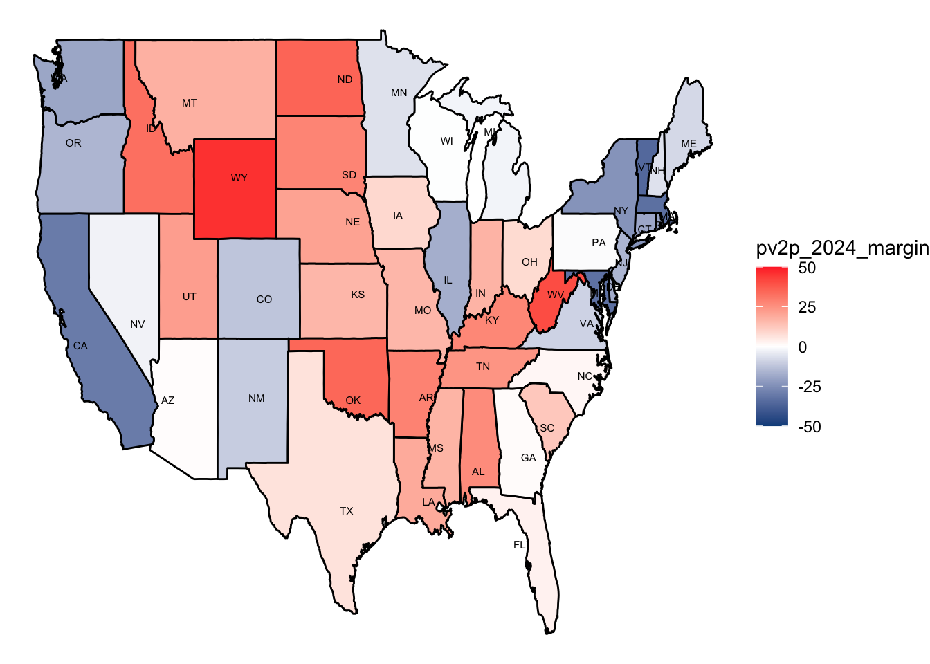
In regard to the second question for this week about which states vote blue/red and how consistently. This graph can help support observations I made from the grid map.
States like California, New York, and Illinois are reliable Democratic strongholds. Other states that I did not know but have proven to consistently vote for the Democratic candidate are Washington, Oregon, Wisconsin, Minnesota. Wisconsin is interesting because in the past nine elections, it has voted for the Democratic candidate except for 2016 and yet the margin for the 2024 forecast does not lean heavily toward the Democrats.
You can also see some geographic patterns where northeast and west coast states tend to favor the Democratic candidate. Southern states, rocky mountain states, and great plain states lean toward the Republican candidate.
Notes
- The initials on the states are still a work in progress
- I am able to commit/push to github and create a new post but when it comes to seeing the post on my Hugo site it never shows up. I will be going to office hours this week to resolve this issue. The code for this blog post can be found in my github repository under the name “testPost.Rmd”